Introduction

Signal processing in electrical engineering is used to extract information from electrical circuits. Current and voltage will vary with time, based on the characteristics of the circuit. Signals can be sent along electrical circuits from one location to another. At the final location, these signals must then be processed. This section will go over the basics of signal processing as it relates to the Electrical FE exam. Signal Processing accounts for approximately 5 to 8 questions on the Electrical FE exam. These questions can cover convolution, difference equations, z-transforms, sampling, analog filters and digital filters.

The NCEES FE Reference Handbook contains very basic information on difference equations and convolution. This seems to indicate that any problems on these topics will be more conceptual as opposed to computational. On the other hand, the handbook contains tables for the z-transforms for various functions and tables for various analog filters. So questions on these topics will be more computational. In addition, digital filters use z-transforms heavily, so problems on digital filters will most likely be computational. Lastly, the handbook has information on various sampling methods, so these questions could also be computational. Although sampling is called for in the outline under Signal Processing, sampling is also typically a part of Communications in electrical engineering courses. Thus, there will be some overlap between this section and Section 14.0 Communications.

2.0 CONVOLUTION

The first concept that you must know for the Electrical FE exam Signal Processing topic is convolution. Convolution involves combining two signals to make a third signal. The NCEES outline specifically calls out two methods of convolution, (1) continuous time and (2) discrete time.

Discrete Time: A discrete time signal is shown by pulses at various points of time.

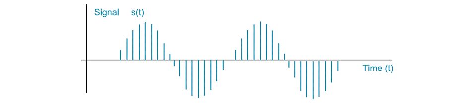
Figure 1: A discontinuous aka discrete time signal is shown by this figure. The signal has breaks, meaning there isn’t a y-value for every x-value (any point in time).

Continuous Time: A continuous time signal is shown by a continuous pulse that can vary its amplitude over time.

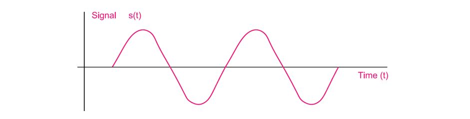
Figure 2: A continuous time signal is shown by this figure. The signal has no breaks, meaning there is a y-value for every x-value (any point in time).

Convolution is a mathematical operation involving the input signal, impulse response, and output signal.

Continuous-Time Convolution

The convolution of continuous signals in the time domain is represented by the equation below. Do not confuse the "*" symbol for a multiplication symbol. Instead, the symbol is another mathematical operation that means the two functions, x(t) and h(t), are integrated with the following format. Pay attention to the exam questions. If it asks you to find the convolution of signals, then you should know to use this equation.

Convolution of the continuous time function can also be depicted by the block diagram below.

Figure 3: Block diagram of a continuous-time convolution with input x(t), impulse response h(t), and output y(t).

To better understand what is going on, let us first define h(t). In the equation above, h(t) is the impulse response of a linear, time invariant system. If you were to send a unit impulse signal through a system, the output would be the impulse response. (Refer to Section 8.0 Linear Systems for the definition of a linear system. A time invariant system means that it does not matter when you send a signal through a system, the output will be the same. A unit impulse is a sharp spike in a signal, infinitely tall with the area under its curve equal to one.)

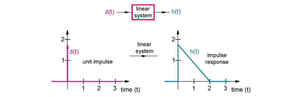
Figure 4: Example of an impulse response. A unit impulse δ(t) is sent through a linear system and the output is the impulse response.

An impulse response can be used to characterize a system. Because the system is linear and time invariant, the impulse response can be used to determine the output of any input into the system. So, if the input were a function, x(t), it could be broken up into a bunch of impulses that were sent through the system. Then, the output of each impulse added up together would equal the convolution, y(t), or essentially the output of x(t).

The best way to understand how the convolution equation is used is to complete an example.

The equation format of convolution is a little confusing, it is better explained graphically. The operation is graphically performed by sliding one function over another function along the x-axis, moving from left to right. The function that slides goes from negative infinity to positive infinity, while the other function remains still. As the two functions overlap, the area of the overlap at each instance in time is graphed as the output y(t). This is illustrated by the example below.

Let the input x(t) and the impulse response h(t) be defined by the following functions. The first step is to set up the equations in graphical format.

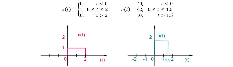
Figure 5: Graph and corresponding function of input x(t) and impulse response h(t).

Then, replace time t with a dummy variable that is shown in the convolution equation as τ. We need a dummy variable for the x-axis because the time t variable will be used to slide the h(t) function as τ remains as is.

Figure 6: The variable t is replaced with the dummy variable, τ.

Next, replace the variable in the h(t) function with (t – τ). Graphically this means that h(t) will be flipped along the y-axis, since τ is now negative. The figure below shows h(t) at time t=0.

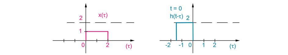
Figure 7: The next step is to create function, h(t- τ). Since there is a negative sign, the graph h(t) was mirrored around the y-axis. This figure shows h(t- τ) when t = 0. If t is negative, then the graph will be shifted to the left, if t is positive then the graph will be shifted to the right.

Finally, the following figure shows the convolution of x(t) and h(t). The top part of the figure shows h(t-τ) in blue moving from left to right, as time, t, goes from negative infinity to positive infinity. When the two functions coincide, the convolution area is calculated as the magnitude of the x function multiplied by the magnitude of the h function across the width of intersection. This area is shown as the shaded region. Since x and h both have magnitudes of 1 and 2 respectively, the convolution area has a height of 1*2=2. The bottom figure graphs the area at each point in time.

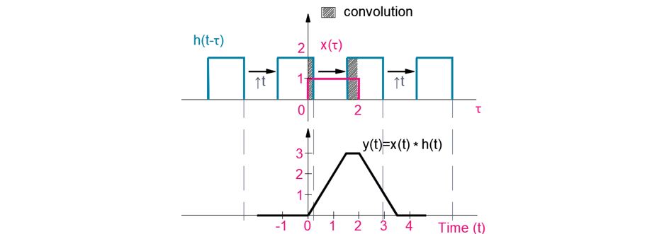
Figure 8: The top figure shows the progression of the convolution process and the bottom figure shows the result of the convolution process along time, t.

Hopefully, convolution is becoming clearer, but for additional clarity the same convolution process is conducted in a case by case basis.

This section is continued in more detail in the technical study guide . Also included are many more practice exam problems.

3.0 Z-TRANSFORMS

A Z-transform is used to convert discrete signals in the time domain to a complex (real & imaginary) Z-domain. The Z-domain is essentially a discrete version of the frequency domain. The Z-transform is similar to the Laplace transform, but uses discrete time signals instead of continuous, which is why you will see similar Z-transform pairs as the Laplace transform pairs, which will be discussed in the next part of this section.

The variable z is defined as the complex number in terms of frequency, ω, below.

To illustrate how the Z-domain represents a signal as a complex number, a graphical comparison of the various planes is shown below. This is a simplified view and is only intended to give you a visual context of the transformations being performed. The actual graphing process between domains is likely more in depth than what is required for the exam.

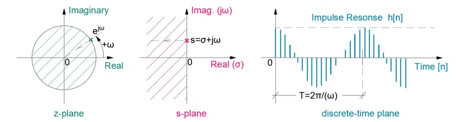
Figure 9: A simplified comparison of the z, s, and time domains are represented in the graph above. The s and z plots are shown as a point (complex number) on their respective planes, for |z| is equal to 1. The shaded region in the z and s-plane is considered the stable region. Anything outside of it is unstable, which means that z will have a magnitude greater than one and h[n] will continuously increase with time. If z was less than 1, h[n] would converge as time increased.

Similar to the Laplace transform, the Z-transform is used to simplify the calculations of complex equations. Instead of differential equations being converted to algebraic equations in the s-domain, difference equations are converted to algebraic equations in the Z-domain. The calculation is performed in the Z-domain, then converted back to the time domain. Difference equations are the discrete equations and described later in this section.

The Z-transform of a discrete function, f[n], is written as F(z).

The equation for the Z-transform is written out below. In this equation you take the sum of each discrete data point, multiplied by the z factor shown. This equation is called the unilateral z-transform because it is summed from only the positive side of the graph.

This following equation is called the bilateral z-transform because it is summed from negative infinity to positive infinity.

The inverse of the z-transform is shown below. The integral is taken within the closed contour, Γ. This calculation can be difficult to perform, so instead the z-transform pairs are used.

Z-Transform Pairs

On the FE exam, you should be familiar with the z-transform pairs presented in the NCEES FE Reference Handbook. This section will go into more detail into how to use that table.

Delta Function

The first transform pair is of the delta function or impulse signal. The delta function here is a discrete impulse signal. Where the continuous impulse signal previously mentioned has a height of infinity, a width infinitesimally small, and area equal to 1, the discrete impulse signal is equal to 1 at n=0. The equation and graph are shown below.

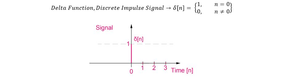
Figure 10: The impulse delta function is unity at n = 0. This figure shows the discrete version. The function is 0 at all other x-values.

The Z-transform of the delta function is simply equal to 1.

Step Function

The second transform pair is of the step function. The step function and graph are shown below. The step function is equal to 1 at all points greater than or equal to n = 0. It is 0 everywhere else.

Figure 11: The step function is shown in this figure.

The Z-transform of the step function is equal to the following equation.

Exponential Function

The third transform pair is of the exponential function. The exponential function is multiplied by the step function, so that it is only valid for time “n” greater than or equal to 0. The exponential function is raised to a constant alpha multiplied by time.

This section is continued in more detail in the technical study guide . Also included are many more practice exam problems.

4.0 DIFFERENCE EQUATIONS

A difference equation is an equation that uses the past inputs to determine the present input. For example, if you are at a time t = 3 seconds, then a difference equation for t = 3 seconds would be based on the values at t = 2 seconds and t = 1 seconds. The equation for time t = 4 seconds would be based on the values at t = 3 seconds and t = 2 seconds.

Example: In this example, the amplitude of the signal, y[n], is dependent on the x[n], x[n-1] and x[n-2]. The signal is dependent on the values of the function x at the current time and previous times.

The difference equations will lead to the filter section.

The first order difference equation is shown in the following format in the NCEES FE Reference Handbook.

This section is continued in more detail in the technical study guide . Also included are many more practice exam problems.

5.0 ANALOG FILTERS

Multiple signals with varying frequencies can be sent over a transmission medium. Analog filters are used to isolate signals with specific frequencies. The analog filters covered in the NCEES FE Reference Handbook are (1) First Order Low Pass Filter, (2) First Order High Pass Filter, (3) Band-Pass Filter and (4) Band-Reject Filter. Filters were also introduced in the 8.0 Linear Systems Section, under frequency response.

First Order Low Pass Filter

An analog filter that passes all signals below a certain frequency is a low pass filter, because it allows everything lower than the cutoff frequency and blocks anything above the cutoff frequency. Electrically a first order low pass filter consists of an inductor in series with a resistor. The inductor will attenuate higher frequencies and allow lower frequencies through the circuit with less impedance.

This figure shows a low pass filter.

The relationship between the output and input voltage can be found with the basic voltage divider rule. But in order to use that rule you need to convert the components to impedance.

This section is continued in more detail in the technical study guide . Also included are many more practice exam problems.

6.0 SAMPLING

Sampling is the process of converting an analog (continuous time) signal into a digital (discrete time) signal. Sampling is a collection of samples. One sample is an amplitude and a certain point in time.

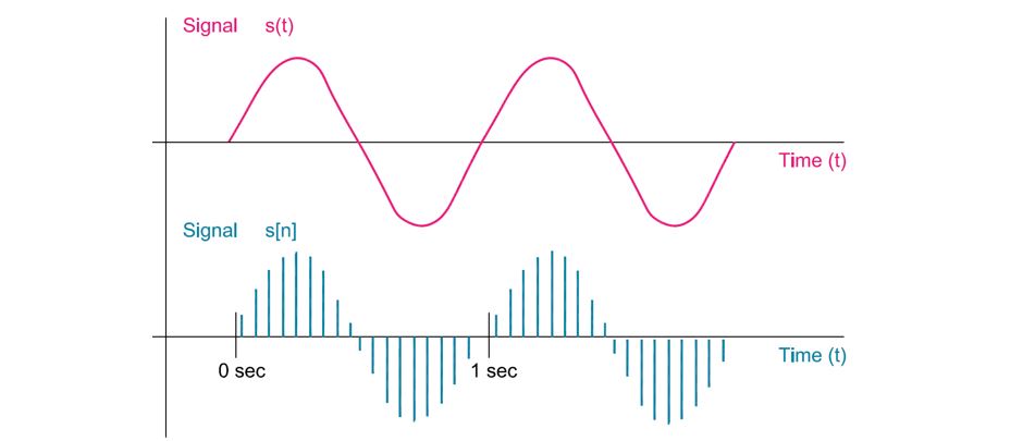
This figure shows how a continuous sine wave can be sampled. The figure shows that in one second there are 18 samples.

The sampling frequency in units of Hertz is equal to the number of samples per second. So in the figure above, the sampling frequency is 18 Hz. The sampling frequency is important because too little samples may not appropriately represent the wave and too many samples may cause an inefficient use of data.

This section is continued in more detail in the technical study guide . Also included are many more practice exam problems.

7.0 DIGITAL FILTERS

This section is continued in more detail in the technical study guide . Also included are many more practice exam problems.

8.0 Practice Problems

8.1 PRACTICE PROBLEM 1 –

8.2 PRACTICE PROBLEM 2 –

8.3 PRACTICE PROBLEM 3 -

Practice Problems 4 through 6 and all solutions are included in the technical study guide, along with many more practice exam problems.