1.0 Introduction

Linear Systems accounts for approximately 5 to 8 questions on the Electrical FE exam. The Linear Systems topic on the NCEES exam covers frequency response, transient response, resonance, Laplace transforms, transfer functions & 2-port theory. Linear Systems also overlaps with NCEES FE Electrical topic called Control Systems. Control Systems moves closer to application in electrical engineering, while this Linear Systems topic focuses more on the mathematics side of control systems.

The NCEES FE Reference Handbook Electrical Engineering section has some basic equations for the topics below, but it does not explain the skills and concepts necessary to use these equations. The Laplace Transform tables are located in the Mathematics section. The resonance equations are located in the Electrical & Computer Engineering section, along with the Two-Port Theory equations. If you like to use the search function you can search the keywords, Laplace, Frequency, Resonance and Two-Port.

2.0 FREQUENCY & TRANSIENT RESPONSE

There are two ways to look at the response of your system, (1) Transient and (2) Frequency. The frequency response looks at the response of your system in the frequency domain and the transient response focuses on the time domain. Transient response occurs when there is a change in a system and it is not yet at steady state. There are two main transient response concepts that you should understand for the exam, since these concepts are shown in the NCEES FE Reference Handbook under the Electrical & Computer Engineering section. These concepts revolve around the RL and RC circuits, shown in the next two parts.

RL Transient Response

The resistor-inductor (RL) circuit consists of inductors (L) and resistors (R). The circuit will respond to a sinusoidal voltage input, based on its inductance and resistance values. Resistors will only affect the circuit by its ohm value. Inductors will responds to the rate of change in current. As current is quickly decreased, the inductor will produce more voltage, in its release of stored energy from its magnetic field to try to keep current constant. If current is slowly decreased, the inductor will produce relatively less voltage, by releasing less stored energy from its magnetic field, to try and keep the current constant. This is seen by the equation V_L (t)=L*(dI/dt).

Figure 1: This circuit shows a switch that is activated at time t = 0 seconds. When the switch is activated, the sinusoidal (AC) voltage source will be connected to the resistor and inductor in series.

The charging and discharging portions shown in the inductor current/voltage versus time graph represent the transient response regions; see the figure below. The governing equation for the current through this circuit, after the switch is latched at time t = 0, is shown by the equation below.

Most times, the initial value will be equal to zero, so the above equation can be simplified to the following equation.

The voltage across the resistor will now be a function of the current multiplied by the resistance value.

The voltage across the inductor will be the voltage source minus the voltage across the resistor.

On the actual FE exam, you may have to simplify complex circuits and put it into the same resistor-inductor format as the one shown in the RL circuit figure above. This will require an understanding of the Thevenin techniques, but will allow you to use the voltage equation above. Another question that could be asked is to find the time constant of the circuit. The time constant is found through the below equation.

The time constant represents the amount of time it takes to store energy in the inductor. At time t=τ, the exponent becomes e^(- 1)=0.368. This means if a constant DC voltage source is applied, then at 1 time constant, the voltage across the inductor will be 36.8% of the source voltage and the current through the circuit will be 63% of the current through the circuit. At time t=5*τ, the current will be 99.3% of the max current. The current will very slowly increase from there, so the inductor will essentially be at steady state.

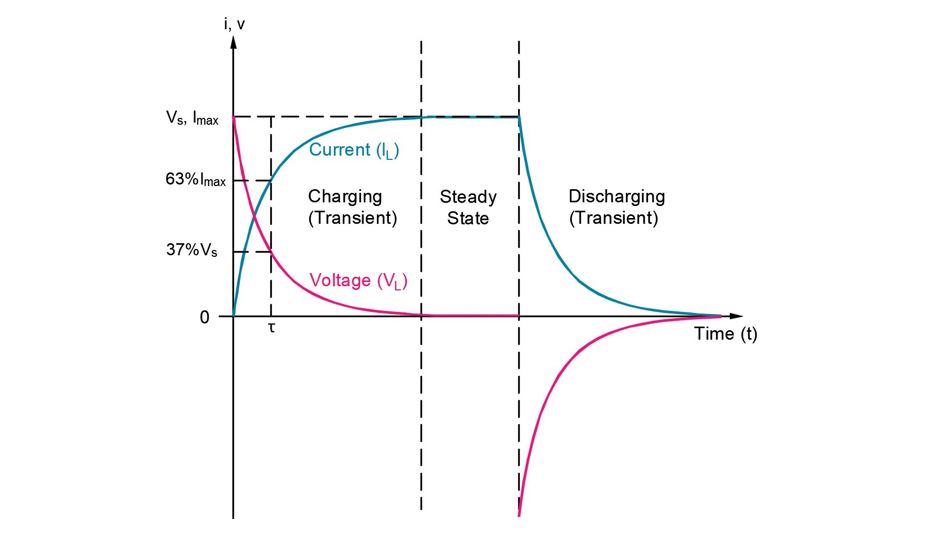
Figure 2: The graph shows current and voltage across an inductor as it is in its transient and steady states. The current will be at 63% when time is equal to the time constant, τ=L/R.

The other way to look at inductors is the previously mentioned equation from the basic circuits section, where it states that the voltage across an inductor is equal to the inductance multiplied by the change in current.

RL Frequency Response

The RL circuit can also be analyzed in the frequency domain. In the frequency domain the resistor and inductor will respond differently to various frequencies. The impedance of the resistor and inductor equations are shown below. These equations show that as the frequency increases, the impedance of the inductor will increase and as the frequency decreases, the impedance of the inductor will decrease. This is why at DC voltage (frequency = 0), the inductor has 0 impedance and acts like a short circuit.

RL circuits can also be used to create high pass and low pass filters using frequency response. The important relationship to know is the cutoff frequency, f_c. This is the frequency that the circuit is intended to filter to. The cutoff frequency for an RL circuit is shown below.

For a low pass filter, frequencies lower than and up to the cutoff frequency are sent to the load. The higher frequencies are filtered out and not let through. The figure below is a very simple example of a low pass filter, where the load is connected across the resistor of an RL circuit.

Figure 3: Low pass filter where the output is connected across the resistor of an RL circuit.

As seen in the previous impedance equation for inductors, ZL, the impedance across an inductor is low when frequency is low. If the impedance across the inductor is much lower than the resistor, most of the source voltage will be distributed across the resistor, i.e. low frequency will send an output voltage across the resistor, high frequency will be filtered out.

A high pass filter uses the fact that the voltage across the inductor will behave opposite of the resistor. So a high pass filter connects the load across the inductor as shown below, allowing frequencies from the cutoff frequency and higher to be sent out.

Figure 4: High pass filter where the output is connected across the inductor of an RL circuit.

Additional discussion on filters can be found in Section 9.0 Signal Processing.

RC Transient Response

The resistor-capacitor (RC) circuit consists of capacitors (C) and resistors (R). The circuit will respond to a sinusoidal voltage input, based on its capacitance and resistance values. Resistors will only affect the circuit by its ohm value. A higher resistance will cause less current and a higher voltage drop. Capacitors will respond to the rate of change in voltage. As voltage is quickly decreased, the capacitor will produce more current, in its release of stored energy to try to keep voltage constant. If voltage is slowly decreased, the capacitor will produce relatively less current, by releasing less stored energy, to try and keep the voltage constant. As a reminder, this is seen by the equation, i_c (t)=C*(dV/dt).

This section is continued in more detail in the technical study guide. The practice exam contains many more practice exam problems.

3.0 RESONANCE

Resonance in an RLC circuit occurs at a frequency when the inductive and capacitive reactance are equal in magnitude and cancel each other out because they are 180 degrees apart in phase. Section 11.0 Power shows how the inductor (L) and capacitor (C) are out of phase by 180 degrees.

The frequency references the time period of the sinusoidal voltage and current waveforms. Frequency can be written in Hertz or in radians per second. Resonant frequency is written as subscript 0.

The impedance of the inductor will increase as the frequency increases and be in the positive imaginary direction, Z_L=jωL (Ω). The impedance of a capacitor will decrease as the frequency increases and be in the negative imaginary direction, Z_C=-j/ωC (Ω). The impedance of a resistor will not vary based on the frequency, Z_R=R (Ω).

There will be a certain frequency that will cause the positive reactance (imaginary impedance) due to the inductor to be canceled out by the negative reactance (imaginary impedance) due to the capacitor. At this resonant frequency, the capacitor will charge while the inductor discharges and the inductor will charge when the capacitor discharges. This will eliminate the effects from the capacitor or inductor, i.e. they will not contribute impedance.

The calculation of the resonance frequency will depend on the circuit arrangement. For the FE exam, there are two circuit arrangements: (1) series and (2) parallel.

Series RLC Resonance

The series RLC circuit configuration is shown below. As the current at resonant frequency cycles back and forth between the inductor and capacitor in a RLC circuit in series, their impedances cancel each other out, acting like a short between inductor and capacitor. The only impedance in the circuit will be due to the resistor, which causes a spike in the current.

Figure 5: This RLC circuit shows an inductor and capacitor in series with a resistor.

In series, the impedances add. To cancel the impedances, the sum must equal zero. Since the inductor and capacitor are in the imaginary component and the resistor is in the real component, the resistor does not affect the calculation. Therefore, the equation at resonant frequency can be simplified to the following.

Solve for the resonant frequency.

At resonance, the impedance will be at its lowest (Z=R), which means the current and thus power through this circuit will be at its highest. If the frequency is varied from this peak, either up or down, then the current and power will decrease.

The quality factor, Q, of the RLC circuit describes how narrow the bandwidth of the resonant frequency is or how high the current spike is. Once the power decreases to a point that is –3 dB down from its maximum, this will define the edge of the bandwidth. This –3dB is a power level and it occurs when the current or voltage is 1/√2 = 0.707 of its maximum value and when the actual power value is 0.5 of its maximum value. It is also the point at which the cutoff frequency that was previously mentioned in high/low pass filters occurs.

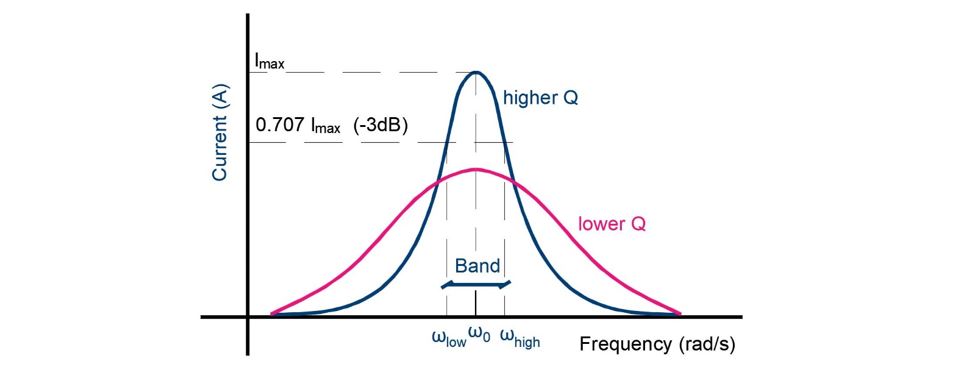
Figure 6: An example of a graphed bandwidth, where ω_high and ω_low are found where the current is 0.707 times the max current or -3dB, which is equivalent to half the max power. The bandwidth shown is for the higher Q curve. The lower Q curve is an example of lower quality factor, which means larger bandwidth.

The high and low frequency can be found with the following equations.

The difference between the high and low frequencies is called the bandwidth.

This also leads to the quality factor, Q.

Additional discussion on bandwidth is found under the Analog Filters topic of Section 9.0 Signal Processing.

Parallel RLC Circuit

In a parallel circuit, resonance also occurs when the impedance from the inductor cancels out the impedance from the capacitor. When the current cycles back and forth between the inductor and capacitor it is isolated to the last loop in the figure below, simulating an open circuit at this leg. Then, current from the source voltage will only flow through the resistor, causing the circuit impedance to be at its peak and the current to be at its minimum.

Figure 6: This RLC circuit shows an inductor and capacitor in parallel with a resistor.

This section is continued in more detail in the technical study guide. The practice exam contains many more practice exam problems.

4.0 LAPLACE TRANSFORMS

Laplace transforms allow you to find the frequency or transient response of linear systems. The Laplace transform will convert difficult differential equations from the time t-domain to the frequency s-domain. Once the equations are in the s-domain, the equations are converted to algebraic equations and become much easier to solve. The s-domain equations can then be converted back to the time domain. The Laplace transform is used in many electrical engineering topics like controls, circuits and electronics.

The following formula shows how you would convert from the time domain to the s-domain. This is the Laplace transform. Note that the constant from the integral must be given to solve these problems.

The following formula shows how you would convert from the s-domain back to the t-domain. This is called the inverse Laplace transform.

A simple example is finding the Laplace transform for the function f(t)=1,where t≥0.

Step Function

On the exam, the previous transformation is the same as the step function equation. A step function is shown in the following figure, where there is a jump in the function. The unit step function goes from 0 to 1, starting at t=0.

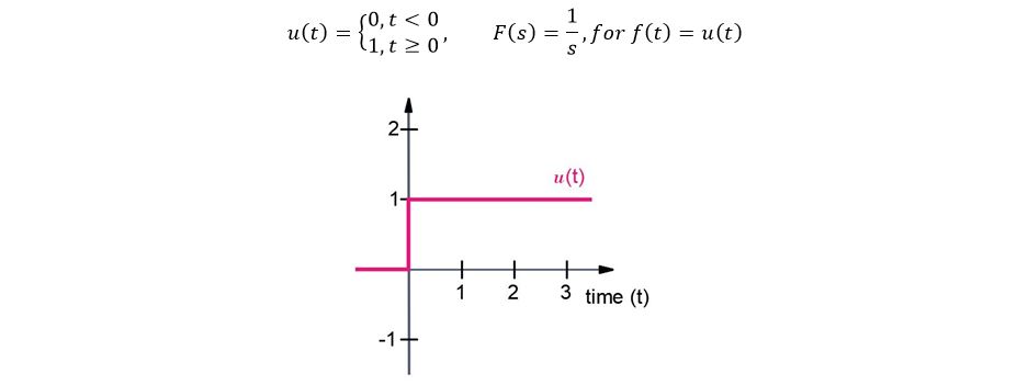
Figure 7: Unit step function for u(t).

Impulse Function

Impulse is when there is an immediate spike at a singular point in time. In this case, the impulse function, δ(t) occurs at time t=0. A unit impulse with a width equal to 0 and an infinite height has an area equal to 1.

Then, because the function only has non-zero value at time t=0, the equation can be rewritten as the following.

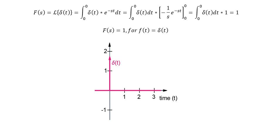
Figure 8: Impulse function for δ(t).

. . .

Laplace Properties

The Laplace properties are used on the exam to simplify complex functions into easy to use functions. These easy to use functions should preferably be in a format listed in the Laplace transform table of the NCEES FE Reference Handbook.

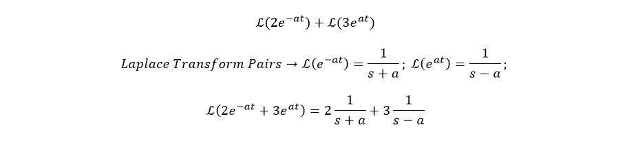
Linearity property

The Linearity property states that you can add two functions and multiply each of those functions by a scalar, then take the Laplace transform of that combined function and it will equal the Laplace transform of each individual function added together.

The linear property is very useful on the exam because you can take a complex function and break it up into the sum of two or more functions. Then, you can take the Laplace transform of each individual function and add the Laplace transforms of each. The following shows a simple example as to how to use this property.

The function can be broken up into two different functions and the Laplace transform of each individual function can be found.

First, Second & Nth Derivative

The Laplace transform of the first derivative of a function is equal to the Laplace transform of the original function multiplied by s. There is also a term for the initial condition at time t = 0.

The second derivative is equal to the Laplace transform of the original function multiplied by s squared. There are now two terms that include the initial condition. The difference is that one of the terms is multiplied by s.

The ultimate pattern is shown on the NCEES FE Reference Handbook. It is labeled as the nth derivative property. Take the Laplace transform of the original function, then multiply that term by s raised to the nth power. Next, you subtract the initial condition multiplied by s raised to the n-1 power and continue until you reach s raised to the 0th power.

Example: This is one way that you can use this property to solve complex Laplace transforms

First, find the derivatives of this function and the conditions at t=0.

Now, use the formula for the derivative property.

Finally, solve for the Laplace transform of the original function.

This section is continued in more detail in the technical study guide. The practice exam contains many more practice exam problems.

5.0 TRANSFER FUNCTIONS

A transfer function is used in electrical engineering to create an equation or model of a circuit’s output as a function of all the possible inputs.

This section is discussed in more detail in Section 13.0 Control Systems in much more detail. Transfer functions poles & zeroes are only briefly mentioned in this section.

Poles of a transfer function are the frequencies for which the value of the denominator of the transfer function becomes zero. Zeroes are the values for when the numerator of the transfer function becomes zero. The poles and the zeros of the transfer function determine the performance and stability of the function.

This section is continued in more detail in the technical study guide. The practice exam contains many more practice exam problems.

6.0 TWO-PORT THEORY

Two-Port theory in the NCEES FE Reference Handbook covers the following two-port circuit. The left hand side is called the inputs. The right hand side is called the outputs. The two-port circuit is used to create a relationship between the output currents & voltages and input currents & voltages of a complex circuit. The middle portion becomes a black box that represents some complex circuit.

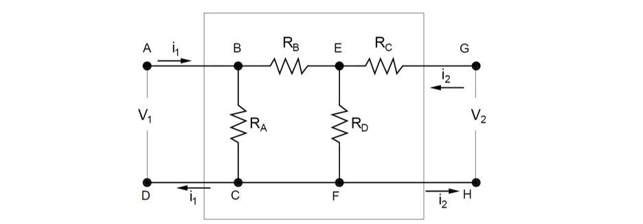
Figure 9: This complex circuit can be represented by a two-port circuit. First, you need to ensure that the current entering the “black box” is equal to the current leaving at both the left side and right side. Once you have the input port (left side A & D) and output port (right side G & H), then you can re-draw the complex circuit as a simple two-port box.

Figure 10: This two-port box represents the complex circuit shown in the previous figure.

The two-port box can then be represented by a voltage and resistance, as shown in the figure below. A common two-port question is to find the equivalent resistances R1 and R2. Other times, the question may ask for the admittance, which is just the inverse of the resistance. This book will show you how to find the equivalent resistances. You can take the inverse of the resistance to find the admittance.

Figure 11: It is very important to note that Voltage 1 (left port) will be reflected by some magnitude “b” onto the right hand side port. Voltage 2 (right port) will be reflected by some magnitude “a” onto the left hand side port.

This section is continued in more detail in the technical study guide. The practice exam contains many more practice exam problems.

7.0 Practice Problems

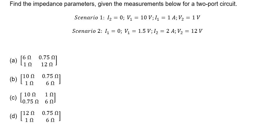
7.1 PRACTICE PROBLEM 1 – 2 PORT THEORY

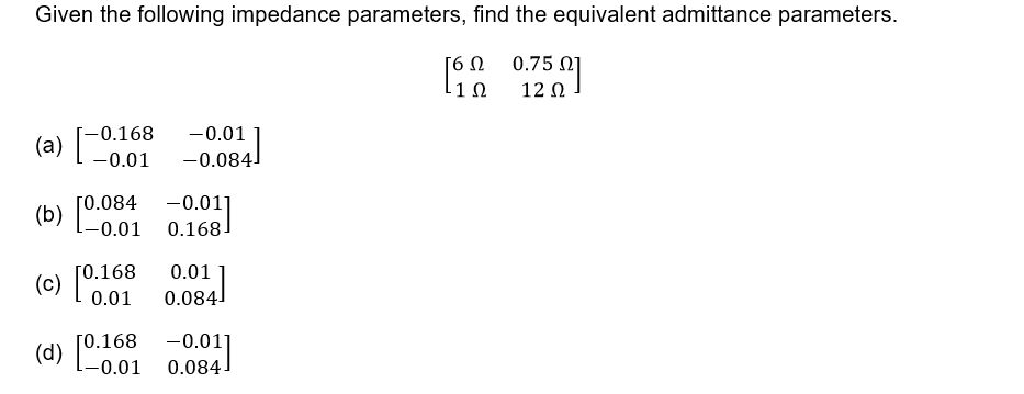
7.2 PRACTICE PROBLEM 2 – 2 PORT THEORY

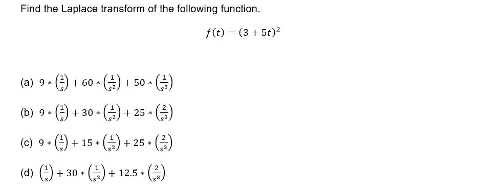
7.3 PRACTICE PROBLEM 3 - LAPLACE TRANSFORM

Practice Problems 4 through 8 and all solutions included in the technical study guide, along with many more practice exam problems.