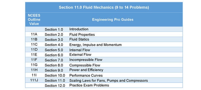
1.0 Introduction

Fluid mechanics accounts for 9 to 14 problems on the Mechanical FE Exam. The topics range from college fluid mechanics topics like fluid properties, fluid statics, energy, impulse, momentum, internal flow, external flow and compressible flow to the topics that are more often used in practice like incompressible flow, power, efficiency, performance curves and scaling laws for fans, pumps and compressors. As you go through this section, you should also check the fluids topics within the NCEES FE Reference Handbook.

2.0 Fluid Properties

During the exam you will need to be able to find and use fluid properties to complete many problems. You should be very familiar with the NCEES FE Reference Handbook and where to find these fluid properties. As you go through these descriptions of the important fluid properties, look through the handbook and you will see that the only fluids mentioned in the handbook with all of these properties are air and water. This should give you an indication that most of the questions on fluids will revolve around air and water and if another fluid is given in a question, then all the properties for that fluid must be provided in the question, except for heat capacity for select fluids like air, water, ethane, methane, mercury, etc. Only select fluids have their densities shown in the handbook.

2.1 DENSITY

The density of a substance is its mass per unit volume. For example, density is typically shown as pound-mass per cubic foot or kilograms per cubic meter.

The density of a fluid is measured as a weight per unit volume. Specific volume is the inverse of density and is measured as a volume per unit mass.

2.1.1 IP Conversions

When performing calculations in English units, it is important to distinguish between pound mass (lbm) and pound force (lbf). The mass of an object is measured in pound-mass, similar to the English units of kilograms (kg). Pound-force, on the other hand, is a measurement of weight. It is a unit of force and is used to describe the mass of an object subject to gravity. Pound-force is comparable to the metric force of Newtons.

To perform calculations between pound-mass and pound force, the conversion factor, gc is used. Since gc is merely a unit conversion factor, it can be multiplied or divided anywhere in an equation.

Finally, mass can be represented in terms of slugs, which simplifies the force equations, essentially internalizing the gc conversion factor.

Example: Density relationships in terms of lbm, slug and lbf.

Realize that the densities in the NCEES FE Reference Handbook properties table is given in terms of 〖lbf∙s〗^2/(ft^4 ) or slug/(ft^3 ).

2.2 VISCOSITY

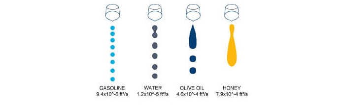
Figure 1: Varying liquids and their viscosities

The viscosity of a fluid describes the fluids resistance to flow. Viscosity is measured in cP or centipoises and is represented by the variable, µ or mu. Viscosity is measured with a device called a viscometer. There are many different types of viscometers, but each typically has the fluid moving past/through an object or it has the object moving through the fluid. The time of travel will vary based on the viscosity of the fluid. For example, water has a viscosity of ~1.00 cP (centipoises) at 68° F, while syrup has a viscosity of ~1400 cP and air has a viscosity of ~.01827 cP.

The units described above are related to cP by a factor of 100. 100 cP is equal to 1 [g/(cm*s)]. The imperial units are[lbm/(ft*s)] and are related to cP by the following conversion.

There are two types of viscosities, dynamic (absolute) viscosity and kinematic viscosity. The previously discussed viscosity µ is dynamic viscosity. Kinematic viscosity describes the ratio of the fluids resistance to flow (dynamic viscosity) to the fluids density. Kinematic viscosity is indicated by the symbol, v or nu.

where ρ=density,μ=dynamic viscosity;v(nu)=kinematic viscosity

Kinematic viscosity has the units ft^2/s as shown above.

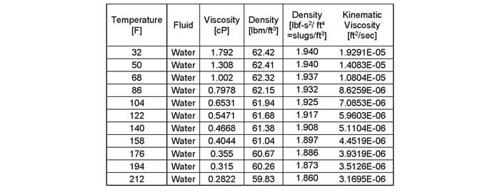
Viscosities of water have been included below for your convenience.

Table 1: This table shows how water’s viscosity and density change as the temperature of water increases.

2.3 SPECIFIC GRAVITY

Specific gravity is the term used to describe the ratio between a liquid’s densities compared to the density of water. Water has a specific gravity of 1.0.

Specific gravity can also be used to describe the ratio between a gas’s densities compared to the density of air. Air has a specific gravity of 1.0.

2.4 HEAT CAPACITY

Heat capacity describes the amount of energy required to raise a fluid’s or solid’s temperature by 1 degree. This term will be discussed more in Section 12.0 Thermodynamics.

There are two types of heat capacity as shown below. The cp term is used for processes involving constant pressure and the cv term is used for processes involving constant volume. The cp term is used to calculate the change in enthalpy of a fluid or solid as a function of a change in temperature of the fluid or solid. Enthalpy includes the For liquids and solids, the terms are very near to one another, because liquids and solids are nearly incompressible. However, for gases the terms will be more different.

2.5 SPECIFIC HEAT RATIO

The specific heat ratio for gases is the ratio of the specific heat capacity at constant pressure and specific heat capacity at constant volume. This is value is used calculate isentropic relationships.

3.0 Fluid Statics

The paragraphs after fluid statics involve fluids in movement. The majority of Section 11 Fluid Mechanics is on moving fluids and not fluids at rest, but there may be a few questions on the FE exam that involve fluid statics. The main concepts that you must understand are the pressure due to fluid height, manometers and buoyancy.

3.1 PRESSURE DUE TO A STATIC FLUID

The first concept that you need to understand is that the static pressure at certain points within a fluid will vary based on the height of the fluid above the point. Static pressure is the pressure acting upon a body or point due to a fluid, when a fluid is at rest.

For example, in the figure below the pressure at point 5A will be greater than the pressure at point 2A, which will be greater than the pressure at point 1A. Another concept that you need to understand is that any container that is open to the atmosphere will have a pressure equal to the atmospheric pressure at that location acting upon the open parts of the container. For example, points 1A and 1B, will have a static pressure equal to the atmospheric pressure and if the location of this container is at sea level, then that pressure will be equal to 14.7 psia. The next concept that you need to understand is that all points at the same elevation will have the same static pressure, for example, points 2A, 2B, 3A, 3B, 4A and 4B will all be at the same static pressure. It may be easier to see how 2A, 3A, 4A and 4B at the same pressure, but maybe not 2B and 3B. It appears that there is not that much fluid acting upon those points, but you need to think about how 2B, 3B and 4B are all at the same pressure. If these points were not at the same pressure then the fluid at point 4B would want to move towards point 3B, but this is not the case because the fluid is at rest.

Lastly, you need to be able to calculate the pressure at each point based on the height of the fluid acting upon that point. Do not forget to include the atmospheric pressure acting upon the top of the fluid, if the container holding the fluid is open.

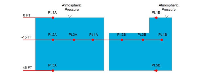
Figure 2: In this figure, all points at the same elevation have the same static pressure. Even though points 2B and 3B do not appear to have the same amount of water acting upon those points, they are at the same pressure as point 4 B. An easy way to think of this concept is that if point 4B was at a higher pressure than point 3B, then the fluid would want to move from point 4B to point 3B, but since the fluid is at rest, then everything at that elevation must be at the same static pressure.

First, you know that the pressure at the top of the container that is open to the surroundings is equal to the atmospheric pressure.

Next, the points 2 through 4, have 15 feet of fluid above these points. In order to calculate the pressure at this point you must convert the weight of the fluid to a force per unit area.

If you make the assumption that the fluid is water, then you can calculate the pressure in terms of pounds per square inch.

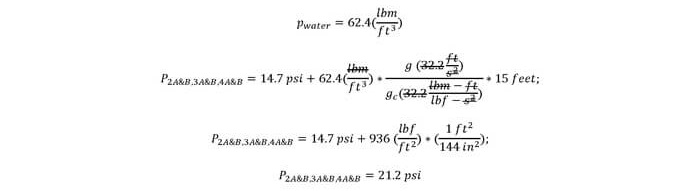
You can then calculate the pressure at the bottom of the container through the same method.

3.2 MANOMETERS

Manometers are used to measure pressures using a tube and a fluid. A fluid medium is placed inside the tube, shown in green in the figure below. One end of the tube is exposed to a fluid of known pressures, indicated as Fluid 3 in the figure below. Typically this fluid is air at atmospheric pressure. The other end of the tube is exposed to the fluid being measured, indicated as Fluid 1 in the figure below. The pressure differential between fluid 1 and 3 can be calculated based on the fluid-medium height difference, using the fluid static principals explained above.

In the figure above, use the equation, ΔP=ρgh to calculate pressure changes from one point to another. Starting from point A and traveling to point B of the tube. Using the density of fluid 1, the pressure difference from point A to point B can be calculated.

Notice that the height at point B is lower than point A, so the pressure will be greater at point B and therefore the pressure shall be added. Now, traveling up from point B to point C, the pressure at point C can be found as the following.

If fluid 3 is air exposed to atmosphere, then fluid 3 and therefore point C and D have a pressure of 14.7psia. The pressure at point A becomes the following.

Manometers can have various configurations, but the principals behind the calculation are the same. Start at one point and add or subtract the pressures based on the vertical height difference of the fluid multiplied by the fluid density and gravity.

3.3 FORCES ON SUBMERGED SURFACES

The following topic discusses how to find the resultant force due to the pressures of a fluid when a flat plat is submerged. The first concept to understand is that the fluid creates a pressure gradient along the plate, which linearly increases as the depth of the submergence, y increases. See the figure below for an illustration of the pressure gradient along a flat plate.

Figure 3: Pressure gradient of fluid acting on a submerged surface

The pressure gradient can be equated to a single resultant force acting on the plate. The magnitude and the location of this resultant force, FR, must be found. The magnitude of resultant force, FR, the moment is taken about a center of rotation, 0. Since the pressure from the fluid is perpendicular to the plate, so is the resultant force. The derived equation for the resultant force is as follows, where P0 is the pressure at the surface and yC is the distance along the plate to the centroid of the area.

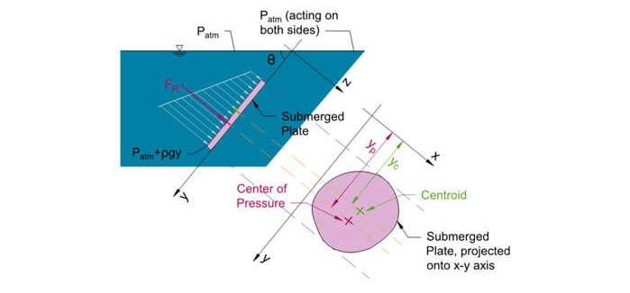
Figure 4: Solving for Resultant Force FR along Submerged Flat Plate

If P0 is atmospheric pressure and the plate is exposed to atmosphere on both sides, then an atmospheric force will be pushing back against FR and the equation becomes:

The position of the reactive force will be located at the center of pressure, and not the area centroid. This is calculated as:

For atmospheric pressure acting on both sides of the surface, P¬0=0, therefore,

Where Ix,C is the area moment of inertia, taken about the centroid along x axis. Find the simplified area moment of inertia equations for typical geometries in the NCEES FE Reference Handbook under statics.

3.4 BUOYANCY

Buoyancy is defined as how a mass sits in a fluid, it either floats or it sinks. The buoyancy force is the force equal to the weight of the volume of displaced fluid. The buoyancy force may be on the exam, but most likely because of how important fluid density is in Thermal & Fluids and how buoyancy force questions test your understanding of fluid density.

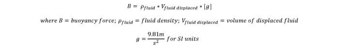
When an object is submerged, the buoyancy force is found through the above equation. Notice that the object’s mass is not in this equation, thus when an object is submerged, the buoyancy force is only dependent on the volume of the object and the density of the fluid.

Figure 5: This shows an object in a fluid, where the object’s weight is greater than the buoyancy force. This causes the object to sink.

When the buoyancy force is equal to the weight of the object, then the object will float.

Figure 6: This shows an object in a fluid, where the object’s weight is equal to the buoyancy force. This causes the object to float.

When the buoyancy force is greater than the weight of the object, then the object will rise.

Figure 7: This shows an object in a fluid, where the object’s weight is greater than the buoyancy force. This causes the object to rise, until it reaches equilibrium, where the object will float.

This section is discussed in more detail in the technical study guide.

4.0 Energy, Impulse & Momentum

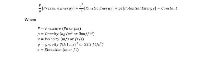
4.1 ENERGY

There are three main types of energy used in fluid calculations, (1) Pressure Energy, (2) Kinetic Energy, and (3) Potential Energy. For steady, incompressible flow, the energy at one point in a system will contain one or more of these energy types. Adding all three components together will yield the total energy at any point in the system, which is found using the following equation known as Bernoulli’s Equation.

Using the conservation of energy principal, the energy at one point can be equated to the energy at another point. Since friction losses are experienced along the way, energy losses due to friction, denoted by the term hf, are also added.

In typical application problems, a pump is sized based on the modified equation below, where the energy added from the work of the pump equals the final conditions of the system.

See the Incompressible Flow topic on how to calculate friction losses.

4.2 IMPULSE-MOMENTUM

The impulse-momentum equations use the principals of Newton’s Second Law, which states that the change in momentum is equal to the external forces acting on an object. For steady flow fluids, this can be analyzed by defining a control volume around the fluid. The sum of all the external forces acting on the control volume will equal the momentum of the fluid entering and leaving the control boundary.

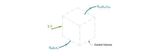
Figure 8: For steady flow fluids, the sum of the changes in momentum in a control volume equals the sum of the external forces acting on the control volume.

...

This section is discussed in more detail in the technical study guide.

5.0 Internal Flow

Internal flow is flow contained within an enclosed boundary, like a pipe or a duct. Internal flow on the FE exam will most likely revolve around finding the pressure drop through these pipes or ducts. In the figure below, fluid enters a pipe with a uniform velocity profile, indicated by the velocity vectors, u, at the entrance. As friction is experienced on the inner surface of the pipe, a velocity profile will be created, where the velocity is 0 at the pipe surface due to friction, and is largest at the center-line of the pipe, which is farthest away from the pipe wall and therefore is able to move more freely. This profile develops after traveling a certain distance in the pipe. When the profile no longer continues to change, the flow is said to be fully developed. This image illustrates how fluid will flow through a pipe.

Figure 9: Internal flow is characterized by a fluid flowing within a pipe or duct.

...

This section is discussed in more detail in the technical study guide.

5.1 REYNOLD’S NUMBER

The Reynold's number (Re) is used to determine the flow characteristic of the fluid, i.e. whether it is laminar (smooth) or turbulent (rough). The Reynold’s number is a unitless number that is found by multiplying the velocity of the fluid through the pipe by the diameter of the pipe and dividing by the kinematic viscosity of the fluid.

...

This section is discussed in more detail in the technical study guide.

5.2 LAMINAR FLOW

The fully developed fluid flow can be characterized as either laminar or turbulent. The way the fluid flows will determine how the calculations should be performed. Laminar flow is the smooth movement of fluid, which is characterized by the Reynold’s Number indicated above. Since the fluid moves in a more predictable pattern, these flows are easier to calculate.

...

This section is discussed in more detail in the technical study guide.

6.0 External Flow

External flow is the flow of a fluid over an object. Similar to internal flow, fluid will begin at an even velocity profile, this is called the free stream velocity and is shown at the beginning of the flat plate below. As the fluid flows over the object, the friction from the surface of the object will create a velocity profile, where the velocity on the surface is 0, and the velocity continues to increase as you move away from the surface.

Figure 10: External flow is characterized by a fluid flowing over a surface.

6.1 REYNOLD’S NUMBER

The Reynold’s number for external flow is similar, except that instead of the internal diameter, D, the Reynold’s number is dependent on the length of the surface for a flat plate and the external diameter for a cylinder or a sphere. The Reynold’s number is used to calculate the drag coefficient of an object.

...

This section is discussed in more detail in the technical study guide.

6.2 DRAG

As a body moves through a fluid (air or water), there are resistive forces that act upon the body, similar to friction. There are two types of drag, surface drag and form drag. Surface drag depends on the smoothness of the force, the friction factor. Form drag depends on the shape of the object as in its aerodynamic shape.

...

This section is discussed in more detail in the technical study guide.

6.3 LIFT

The lift force acts in a direction that is perpendicular to the relative flow. Lift is created due to the difference in pressure on opposite sides of the object. This is because of the difference in velocity between the fluid on the top and the bottom of the object. If the velocity is faster on the top of the object, this will result in a lower pressure and vice versa, if the velocity is slow on the bottom of the object, this will result in a higher pressure. The net pressure effect will then point upwards.

...

This section is discussed in more detail in the technical study guide.

7.0 Open-Channel Flow

Open channel flows pertain to flows that are not in a fully enclosed tube and are instead open to atmosphere at the top surface. Since an open-channel flow cannot be pressurized, pressures and flows are mainly dependent on gravity. The Reynold’s number for channels follow the same equation as that described in the internal flow topic. One important component to distinguish is that the effective diameter will be calculated based on the hydraulic diameter equation, which is based on the surface that comes into contact with the fluid. The hydraulic radius is one-fourth of the hydraulic diameter.

...

This section is discussed in more detail in the technical study guide.

7.1 MANNING EQUATION

For channels with where the depth of the flow is constant, the average velocity is constant. This is characterized as uniform flow. For uniform flow, which is typically obtained with long runs of a channel at a constant slope, the velocity can be found with the Manning equation.

...

This section is discussed in more detail in the technical study guide.

8.0 Compressible Flow

In reality, all fluids are compressible to some extent. A compressible fluid is defined as a fluid that changes in density when the fluid changes in pressure or temperature. On the exam and in practice, a distinction is made between compressible and incompressible fluids because it makes calculations simpler. The majority of the calculations on the exam will be for incompressible flow. The only exceptions will be when the exam clearly indicates compressible flow or when compressible flow is understood to take place in certain conditions. These conditions include any questions on Mach number or nozzles.

8.1 COMPRESSIBLE FLUID

A compressible fluid will reduce its volume in the presence of an external pressure. The quantitative measurement of the compressibility is taken as the relative volume change of the liquid in response for a pressure change.

...

This section is discussed in more detail in the technical study guide.

8.2 MACH NUMBER

Mach number is the ratio of speed to sound. It is a value between 0 and infinity. Transonic, subsonic, supersonic, hypersonic, hypervelocity.

...

This section is discussed in more detail in the technical study guide.

8.2.1 Speed of Sound

The speed of sound in an ideal gas is found through the following equation, which is dependent solely on absolute temperature.

...

This section is discussed in more detail in the technical study guide.

8.3 NOZZLES

Nozzles are used to create changes in velocities and pressures of a moving fluid. A nozzle in its simplest form increases the velocity of a fluid by reducing the area, which also increases the fluids pressure.

...

This section is discussed in more detail in the technical study guide.

8.3.1 Conservation of energy & mass

One important concept to understand for both nozzles and diffusers is that energy is assumed to be conserved as the fluid passes through the nozzle. Any kinetic energy change (change in velocity) must be accounted for in a change in internal energy. For example, an increase in velocity will result in a decrease in temperature and pressure. When solving nozzle equations, you should use these three equations, (1) conservation of energy, (2) conservation of mass and (3) the ideal gas law.

...

This section is discussed in more detail in the technical study guide.

8.3.2 Converging-Diverging Nozzle

A more complex, converging-diverging nozzle consists of a converging portion that is used to raise the pressure of the fluid and then a throat section, followed by a diverging section. The diverging section is a location of low pressure and in application the fluid in the diverging section is typically released into ambient conditions or a tank.

...

This section is discussed in more detail in the technical study guide.

8.4 DIFFUSERS

Diffusers are the opposite of nozzles. Diffusers decrease the pressure of the fluid by reducing the velocity.

...

This section is discussed in more detail in the technical study guide.

8.5 BULK MODULUS

The term Bulk Modulus is a property of a fluid that describes the compressibility of the fluid. Bulk modulus, β, is defined in the equation below.

...

This section is discussed in more detail in the technical study guide.

9.0 Incompressible Flow

As previously discussed, incompressible fluids do not occur in the real world. Incompressible fluids were created to describe a range of fluids, in order to make calculations simpler. The calculations are simpler because incompressible fluids are assumed. An incompressible fluid is a fluid that does not change the volume of the fluid due to external pressure. Most of the basic calculations done in fluid dynamics are done assuming the fluid is incompressible. The approximation of incompressibility is acceptable for most of the liquids as their compressibility is very low. However, the compressibility of gases is high, so gases cannot be approximated as incompressible fluids. The compressibility of an incompressible fluid is always zero.

9.1 FRICTION LOSS – DARCY WEISBACH

Friction loss is found through the use of either the Darcy Weisbach equation or the Hazen-Williams equation. The Darcy Weisbach equation is slightly more involved and will be explained below, starting with the equation. The Hazen-Williams equation is explained in an upcoming topic.

...

This section is discussed in more detail in the technical study guide.

9.2 FRICTION LOSS – HAZEN-WILLIAMS EQUATION

The Hazen-Williams equation is a simplified pressure drop equation that is used in the civil engineering and some mechanical engineering fields. This equation is not accurate for laminar flow and for extremely turbulent flow. The equation is an empirical formulation, meaning that it was created based on experiments and curve fit data. This makes this equation very useful for the typical velocities of 2 to 10 feet per second, because this is the range for which the data fit best.

...

This section is discussed in more detail in the technical study guide.

9.3 FLUID POWER

A large portion of the Thermal & Fluids field is using fluids to transmit power in hydraulic and pneumatic industrial systems. Pneumatics is the transfer of energy via compressed air and hydraulics is the transfer of energy via hydraulic fluid like oil. For example, pneumatics is used in the medical field, construction, manufacturing and packaging. Hydraulic fluids are used heavily in the construction and industrial industries to power large equipment like tractors, cranes, excavators, etc. This section of the book provides you a basic understanding of the engineering principles behind both hydraulics and pneumatics.

10.0 Power and Efficiency

10.1 PUMP POWER

10.1.1 PUMP WORK

The required pump work is calculated from the amount of energy that needs to be added to a system to meet final pressure, velocity, elevation, and to overcome all friction loss requirements. The pump energy is derived from Bernoulli’s Equation, where 2 indicates the most hydraulically remote point in a system and 1 indicates the start point of the pumping system. The friction losses will include any friction losses through piping, fittings, equipment, valves, and other miscellaneous losses.

...

This section is discussed in more detail in the technical study guide.

10.1.2 Pump Efficiency

When calculating pump power, there are two types of efficiencies to consider: (1) Pump Efficiency and (2) Motor Efficiency. Pump efficiency accounts for all the losses from the mechanical components of the pump, such as the inefficiencies from the pump impeller, bearings, seals, etc. The power required to overcome all pump efficiencies is called the pump or brake power. Motor efficiencies account for the electrical losses through the motor coils. The power to overcome the motor efficiencies is called the motor or purchased power. This is the power supplied by the electrical circuits to the motor-pump assembly.

...

This section is discussed in more detail in the technical study guide.

10.2 FAN POWER

10.2.1 Fan Work

Fan work and efficiency follow the same principals as pumps, except that instead of a liquid, the fluid is a gas, typically air. Since air is minimally affected by elevation gains, the potential energy term can be neglected.

...

This section is discussed in more detail in the technical study guide.

10.2.2 Fan Efficiency

Fan efficiencies follow the same process as pump efficiencies. Like pumps, there are two types of efficiencies to consider: (1) Fan Efficiency and (2) Motor Efficiency. Fan efficiency accounts for all the losses from the mechanical components of the fan, such as the inefficiencies from the fan blades, bearings, seals, etc. The power required to overcome all fan efficiencies is called the fan or brake power. Motor efficiencies account for the electrical losses through the motor coils. The power to overcome the motor efficiencies is called the motor or purchased power. This is the power supplied by the electrical circuits to the motor-pump assembly.

...

This section is discussed in more detail in the technical study guide.

10.3 COMPRESSORS

10.3.1 Compressor Work

A common skill, that is required of an engineer, is to determine the work done by the compressor. This work is shown as the difference between the compressor entering enthalpy (H1) and the leaving enthalpy (H2). The equation to determine the work of the compressor is shown below. This equation multiples the mass flow rate by the change in enthalpy between the discharge and suction conditions. This will also be covered in Section 12.0 Thermodynamics, since compressors are key components in refrigeration and power cycles.

...

This section is discussed in more detail in the technical study guide.

10.3.2 COMPRESSOR EFFICIENCY

Each compressor is provided with power, which is typically electricity. The compressor efficiency is found by dividing the actual work output calculated in the previous section by the input electricity power.

...

This section is discussed in more detail in the technical study guide.

11.0 Performance Curves

Performance curves are provided for all centrifugal pumps, fans and compressors. Only fans and pumps are covered in this section, while compressors are covered in more detail in Section 12.0 Thermodynamics.

11.1 FAN CURVES

The fan curve is a graph depicting the various points that the fan can operate. The curve displays the amount of CFM the fan will provide at a given total static pressure. Fans should be selected to operate at the stable region. The stable region is the area on the fan curve where there is a single flow rate [CFM] value for each pressure value. In the unstable region, a pressure value can have multiple CFM values, which will cause the fan system to surge. The stable region also has very little change in CFM for large changes in total pressure.

...

This section is discussed in more detail in the technical study guide.

11.2 PUMP CURVES

Pump curves are created by the manufacturers of the pumps through a series of tests and describe the operating points for a specific impeller diameter and pump type. The curve plots the corresponding flow rates at varying pressure, similar to a fan curve. The graph also shows pump efficiency curves. Points within these curves operate at a higher efficiency than the value shown on the curve and points on the curve operate at the stated efficiency.

...

This section is discussed in more detail in the technical study guide.

12.0 Scaling Laws for Fans, Pumps & Compressors

This section is in reference to the affinity and similarity laws for centrifugal fans, pumps and compressors. These laws do not apply to other types of fans, pumps and compressors. For example, they do not apply to positive displacement pumps or compressors, nor do they apply to propeller fans.

12.1 AFFINITY LAWS FOR FANS, PUMPS & COMPRESSORS

First, if the impeller diameter is held constant and the speed of the fan is changed, then flow rate varies directly with the speed, available pressure varies with the square of the speed and the power use varies with the cube of the speed.

...

This section is discussed in more detail in the technical study guide.

12.2 SIMILARITY LAWS FOR FANS, PUMPS & COMPRESSORS

You may come across these formulas, if you encounter a question that compares two similar fans. These formulas are called the similarity laws. These laws compare similar fans within the same series of fans. The previous formulas compared the original condition and new condition of the same fan. These formulas compare two similar fans, with different diameters. In order to best understand what is meant by same series of fans, visit a manufacturer’s website and you will see various fan series that have varying sizes within the same series. Within a series of fans, a fan with “x” diameter wheel and “y” diameter casing can be compared to another fan in the same series of fans, but with “2x” diameter wheel and “2y” diameter casing. The second pump is similar but has twice the diameter of the first fan.

...

This section is discussed in more detail in the technical study guide.

12.3 MULTIPLE FANS OR PUMPS

There will be times when fans are run in conjunction with each other. It is important for the engineer to understand how the performance is affected depending on the different arrangements of multiple fans. Please refer to Section 15.0 Mechanical Design and Analysis for this discussion.

13.0 Practice Problems

13.1 PRACTICE PROBLEM 1 – VISCOSITY

Honey has a dynamic viscosity of 1,000 poise, a specific heat capacity of 0.6 cal/g-oC, and a density of 0.05 oz/mL. The kinematic viscosity of honey, in ft2/sec, is most nearly?

(A) 0.76

(B) 7.1

(C) 25

(D) 30

13.2 PRACTICE PROBLEM 2 – PIPE FLOW

50 GPM of water flows through a 2-1/2" pipe and then branches into (2) pipes shown in the figure below. If the velocity in the 1-1/2" pipe is measured at 4 ft/sec, then what is the velocity through the 1" pipe?

(A) 3.9 ft/sec

(B) 5.6 ft/sec

(C) 7.2 ft/sec

(D) 9.1 ft/sec

13.3 PRACTICE PROBLEM 3 – REYNOLDS NUMBER

This section is discussed in more detail in the technical study guide.

13.4 PRACTICE PROBLEM 4 – PRESSURE DROP

This section is discussed in more detail in the technical study guide.

13.5 PRACTICE PROBLEM 5 – REYNOLDS NUMBER

This section is discussed in more detail in the technical study guide.

13.6 PRACTICE PROBLEM 6 – FRICTION LOSS

This section is discussed in more detail in the technical study guide.

13.7 PRACTICE PROBLEM 7 - BUOYANCY

This section is discussed in more detail in the technical study guide.

13.8 PRACTICE PROBLEM 8 – PRESSURE DROP

This section is discussed in more detail in the technical study guide.

13.9 PRACTICE PROBLEM 9 – IMPULSE MOMENTUM

This section is discussed in more detail in the technical study guide.

13.10 PRACTICE PROBLEM 10 – IMPULSE MOMENTUM

This section is discussed in more detail in the technical study guide.

13.11 PRACTICE PROBLEM 11 – COMPRESSOR

This section is discussed in more detail in the technical study guide.

13.12 PRACTICE PROBLEM 12 – POWER AND EFFICIENCY

This section is discussed in more detail in the technical study guide.

13.13 PRACTICE PROBLEM 13 – PERFORMANCE CURVE

This section is discussed in more detail in the technical study guide.

13.14 PRACTICE PROBLEM 14 – SCALING LAWS

This section is discussed in more detail in the technical study guide.

13.15 PRACTICE PROBLEM 15 – EXTERNAL FLOW

This section is discussed in more detail in the technical study guide.

13.15 PRACTICE PROBLEM 16 – COMPRESSIBLE FLOW

This section is discussed in more detail in the technical study guide.